

Duplicate information might be useful sometimes, but in most of the cases, it makes the understanding of our data hard and not usable. Here we will take a look at how to easily spot Duplicate Data and Remove it from our Excel Spreadsheet!
Highlight Duplicate Cells
First, we are going to look at How to Highlight Duplicate Cells in order to find them easily. This is an easy 3 step process:
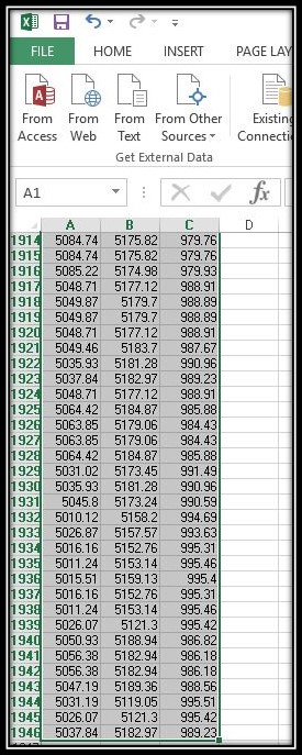
- We have to select all the cells we want to Analyze.
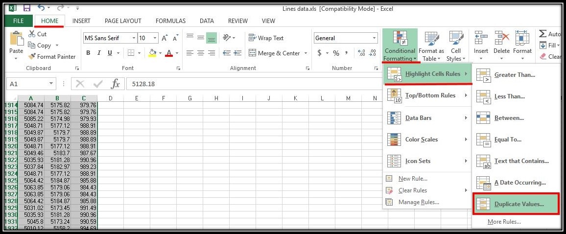
- Secondly, we will click on Home > Conditional Formatting > Highlight Cells Rules > Duplicate Values.
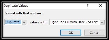
- A window will pop up called Duplicate Values, here next to the values with we can pick the formatting we want and then hit OK.
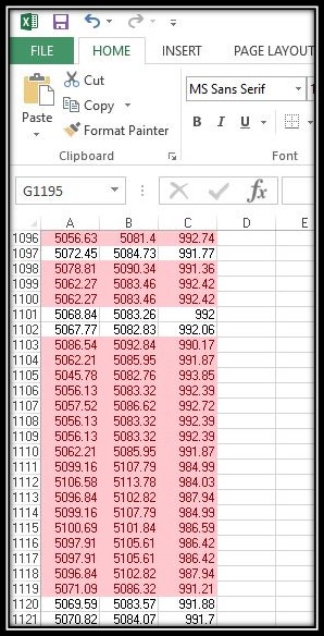
As you can see most of the data in our Example is Duplicate. Now we can decide whether or not we need those duplicates.
Remove Duplicate Cells in Excel
Removing Duplicate rows is as easy as highlighting them. Again we will go through 3 simple steps:
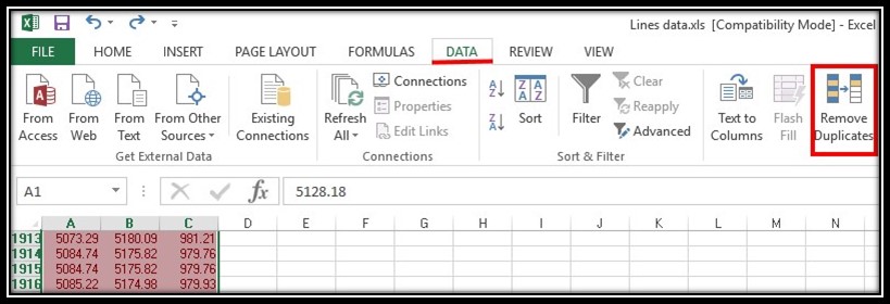
- First, select cells that have duplicate values we want to remove
- Secondly, we click on the Data tab and then Remove Duplicates.
- A window will pop up, here we will check the columns where we want to remove the duplicates. After that, we hit OK.
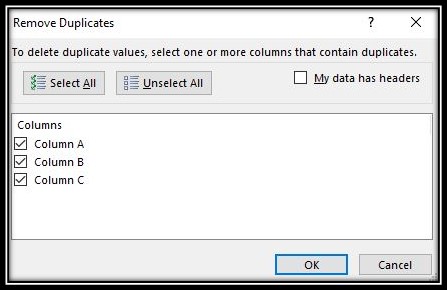

This is the easiest way to Remove Duplicates in Excel with just 3 Clicks of the mouse!
Hope you like the post and find it informative! You can check out our other Microsoft Office Posts!