Flip Columns in Excel – 2 Extremely Quick and Easy Methods!

Many times I myself faced this problem – Flip column data in Excel. It was extremely painful and inefficient to fill all the cells again by hand, that’s why I was so happy when I learned those two tricks!

Flip data upside down using Sort command!

This method requires us to create “help” column besides our data. Then we would use Sort command to reverse the data in our main column. Let’s go through the whole process step by step:

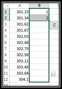
1. We create the “Help” Column next to our main one. The new column must consist of numbers from 1 to X. (the same number as cells in our main column)
   
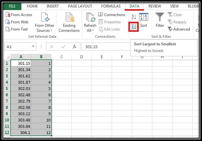
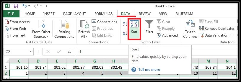
2. Now we have to click on “Sort Largest to Smallest“. The button is located in “Data” ribbon tab under Sort & Filter.
   
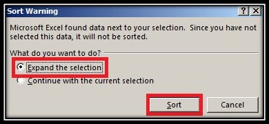
3. After hitting “Sort Largest to Smallest” in the Sort Warning dialog window, we will have to check Expand the Selection and then click Sort.
   

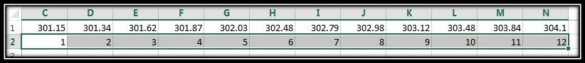
We now have our column revised in order. This method will flip all the columns that are right next to our “Help” column.

Bonus tip: Flip data in rows using sort!

To flip rows, we have to go through identical steps!

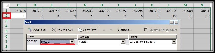
1. We create “Help” row under our main one. The new one again must have numbers from 1 to X.
   
2. This time we hit “Sort” button located again in Data under Sort & Filter tab.
   
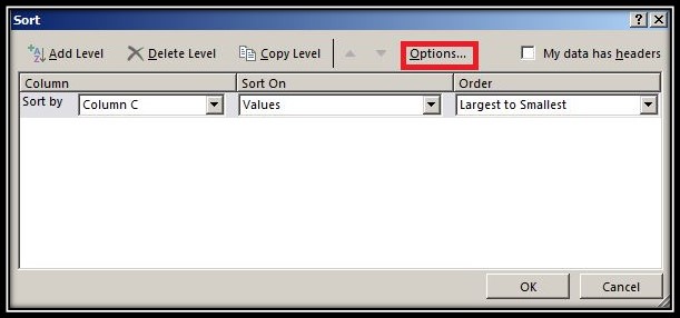
3. Under Sort Warning dialog box we again hit Expand the Selection, but now a new window called Sort will pop up. Here we hit Options… button.
   
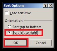
4. Here, we change orientation from “Sort top to bottom” to “Sort left to right”
   
5. In sort window we have to choose our “Help” row in this example we choose “Row 2”
   

Our rows are now Flipped!!

Flip Column in Excel using Formula!

This method requires filling up one simple formula. We will go through the steps again:

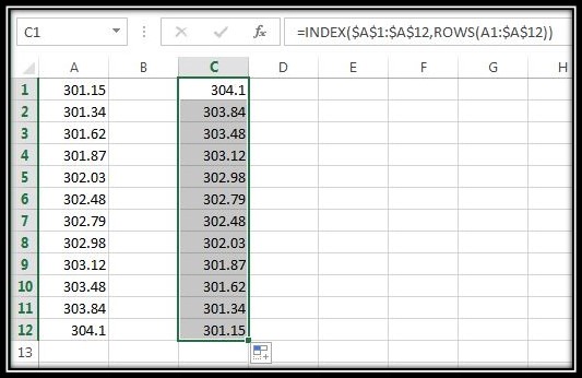
1. We have to fill up this formula =INDEX($A$1:$A$12,ROWS(A1:$A$12)) in the column where we want to flip the data.
   
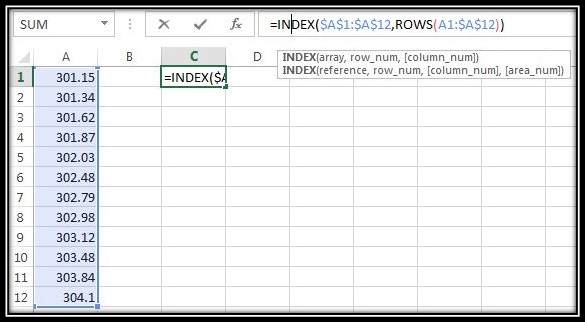
   Note: You have to select your range of cells in the example we are flipping cells 1 to 12 that is why they are used in the formula.
2. After filling up the formula we just have to drag it down until all the cells are flipped!
   

Save hours of typing by using those two simple tricks!